Tensor

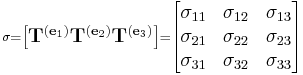 whose columns are the forces acting on the
  ,
,  , and
, and  faces of the cube.
Tensors are geometric entities introduced into mathematics and physics to extend the notion of scalars, geometric vectors, and matrices to higher orders. Tensors were first conceived by Tullio Levi-Civita and Gregorio Ricci-Curbastro, who continued the earlier work of Bernhard Riemann and Elwin Bruno Christoffel and others, as part of the absolute differential calculus. The concept enabled an alternative formulation of the intrinsic differential geometry of a manifold in the form of the Riemann curvature tensor.[1]
Many physical quantities are naturally regarded not as vectors themselves, but as correspondences between one set of vectors and another. For example, the stress tensor T takes a direction v as input and produces the stress T(v) on the surface normal to this vector as output and so expresses a relationship between these two vectors. Because they express a relationship between vectors, tensors themselves are independent of a particular choice of coordinate system. It is possible to represent a tensor by examining what it does to a coordinate basis or frame of reference; the resulting quantity is then an organized multi-dimensional array of numerical values. The coordinate-independence of a tensor then takes the form of a "covariant" transformation law that relates the array computed in one coordinate system to that computed in another one.
The order (or degree) of a tensor is the dimensionality of the array needed to represent it. A number is a 0-dimensional array, so it is sufficient to represent a scalar, a 0th-order tensor. A coordinate vector, or 1-dimensional array, can represent a vector, a 1st-order tensor. A 2-dimensional array, or square matrix, is then needed to represent a 2nd-order tensor. In general, an order-k tensor can be represented as a k-dimensional array of components. The order of a tensor is the number of indices necessary to refer unambiguously to an individual component of a tensor.
Contents |
History
The concepts of later tensor analysis arose from the work of C. F. Gauss in differential geometry, and the formulation was much influenced by the theory of algebraic forms and invariants developed in the middle of the nineteenth century.[2] The word "tensor" itself was introduced in 1846 by William Rowan Hamilton[3] to describe something different from what is now meant by a tensor.[4] The contemporary usage was brought in by Woldemar Voigt in 1898.[5]
Tensor calculus was developed around 1890 by Gregorio Ricci-Curbastro under the title absolute differential calculus, and originally presented by Ricci in 1892.[6] It was made accessible to many mathematicians by the publication of Ricci and Tullio Levi-Civita's 1900 classic text Méthodes de calcul différentiel absolu et leurs applications (Methods of absolute differential calculus and their applications) (Ricci & Levi-Civita 1900) (in French; translations followed).
In the 20th century, the subject came to be known as tensor analysis, and achieved broader acceptance with the introduction of Einstein's theory of general relativity, around 1915. General relativity is formulated completely in the language of tensors. Einstein had learned about them, with great difficulty, from the geometer Marcel Grossmann.[7] Levi-Civita then initiated a correspondence with Einstein to correct mistakes Einstein had made in his use of tensor analysis. The correspondence lasted 1915–17, and was characterized by mutual respect, with Einstein at one point writing:[8]
| “ | I admire the elegance of your method of computation; it must be nice to ride through these fields upon the horse of true mathematics while the like of us have to make our way laboriously on foot. | ” |
Tensors were also found to be useful in other fields such as continuum mechanics. Some well-known examples of tensors in differential geometry are quadratic forms such as metric tensors, and the Riemann curvature tensor. The exterior algebra of Hermann Grassmann, from the middle of the nineteenth century, is itself a tensor theory, and highly geometric, but it was some time before it was seen, with the theory of differential forms, as naturally unified with tensor calculus. The work of Élie Cartan made differential forms one of the basic kinds of tensor fields used in mathematics.
From about the 1920s onwards, it was realised that tensors play a basic role in algebraic topology (for example in the Künneth theorem). Correspondingly there are types of tensors at work in many branches of abstract algebra, particularly in homological algebra and representation theory. Multilinear algebra can be developed in greater generality than for scalars coming from a field, but the theory is then certainly less geometric, and computations more technical and less algorithmic. Tensors are generalized within category theory by means of the concept of monoidal category, from the 1960s.
Definition
There are several different approaches to defining tensors. Although seemingly different, the approaches just describe the same geometric concept using different languages and at different levels of abstraction.
... as multidimensional arrays
Just as a scalar is described by a single number and a vector can be described by a list of numbers, tensors in general can be considered as a multidimensional array of numbers, which are known as its "scalar components" or simply "components." The entries of such an array are symbolically denoted by the name of the tensor with indices giving the position in the array. The total number of indices is equal to the dimension of the array and is called the order or the rank of the tensor.[Note 1] For example, the entries (also called components) of an order 2 tensor T would be denoted Tij, where i and j are indices running from 1 to the dimension of the related vector space.
Just like the components of a vector change when we change the basis of the vector space, the entries of a tensor also change under such a transformation. Recall that the components of a vector can respond in two distinct ways to a change of basis (see covariance and contravariance of vectors),

where Rij is a matrix and in the second expression the summation sign was suppressed (a notational convenience introduced by Einstein that will be used throughout this article). The components, vi, of a regular (or column) vector, v, transform with the inverse of the matrix R,

where the hat denotes the components in the new basis. While the components, wi, of a covector or (row vector), w transform with the matrix R itself,

The components of a tensor transform in a similar manner with a transformation matrix for each index. If an index transforms like a vector with the inverse of the basis transformation, it is called contravariant and is traditionally denoted with an upper index, while an index that transforms with the basis transformation itself is called covariant and is denoted with a lower index. The "transformation law" for a rank m tensor with n contravariant indices and m-n covariant indices is thus given as,

Such a tensor is said to be of order or type (n,m-n).[Note 2]
The definition of a tensor as a multidimensional array satisfying a "transformation law" traces back to the work of Ricci.[1] Nowadays, this definition is still popular in physics and engineering text books.[9][10]
Tensor fields
In many applications, especially in differential geometry and physics, it is natural to consider the components of a tensor to be functions. This was, in fact, the setting of Ricci's original work. In modern mathematical terminology such an object is called a tensor field, but they are often simply referred to as tensors themselves.
In this context the defining transformation law takes a different form. The "basis" for the tensor field is determined by the coordinates of the underlying space, and the defining transformation law is expressed in terms of partial derivatives of the coordinate functions,  , defining a coordinate transformation,

... as multilinear maps
A downside to the definition of a tensor using the multidimensional array approach is that it is not apparent from the definition that the defined object is indeed basis independent, as is expected from an intrinsically geometric object. Although it is possible to show that transformation laws indeed ensure independence from the basis, sometimes a more intrinsic definition is preferred. One approach is to define a tensor as a multilinear map. In that approach a type (n,m) tensor T is defined as a map,

where V is a vector space and V* is the corresponding dual space of covectors, which is linear in each of its arguments.
By applying a multilinear map T of type (n,m) to a basis {ej} for V and a canonical cobasis {εi} for V*,

a n+m dimensional array of components can be obtained. A different choice of basis will yield different components. But, because T is linear in all of its arguments, the components satisfy the tensor transformation law used in the multilinear array definition. The multidimensional array of components of T thus form a tensor according to that definition. Moreover, such an array can be realised as the components of some multilinear map T. This motivates viewing multilinear maps as the intrinsic objects underlying tensors.
This approach, defining tensors as multilinear maps, is popular in modern differential geometry textbooks[11] and more mathematically inclined physics textbooks.[12]
... using tensor products
For some mathematical applications, a more abstract approach is sometimes useful. This can be achieved by defining tensors in terms of elements of tensor products of vector spaces, which in turn are defined through a universal property. A type (n,m) tensor is defined in this context as an element of the tensor product of vector spaces,

If vi is a basis of V and wj is a basis of W, then the tensor product  has a natural basis
  . The components of a tensor T are the coefficients of the tensor with respect to the basis obtained from a basis {ei} for V and its dual {εj}, i.e.

Using the properties of the tensor product, it can be shown that these components satisfy the transformation law for a type (m,n) tensor. Moreover, the univeral property of the tensor product gives a 1-to-1 correspondence between tensors defined in this way and tensors defined as multilinear maps.
Notation
Einstein notation
Einstein notation is a convention for writing tensors that dispenses with writing summation signs by leaving them implicit. It relies on the idea that any repeated index is summed over: if the index i is used twice in a given term of a tensor expression, it means that the values are to be summed over i. Several distinct pairs of indices may be summed this way, but commonly only when each index has the same range, so all the omitted summations are sums from 1 to N for some given N.
Operations
There are a number of basic operations that may be conducted on tensors that again produce a tensor. The linear nature of tensor implies that two tensors of the same type may be added together, and that tensors may be multiplied by a scalar with results analogous to the scaling of a vector. On components, this operations are simply performed component for component. These operations do not change the type of the tensor, however there also exist operations that change the type of the tensors.
Tensor product
The tensor product takes two tensors, S and T, and produces a new tensor, S ⊗ T ,whose order is the sum of the orders of the original tensors. When described as multilinear maps, the tensor product simply multiplies the two tensors, i.e.

which again produces a map that is linear in all its arguments. On components the effect similarly is to multiply the components of the two input tensors, i.e.

If S is of type (k,l) and T is of type (n,m), then the tensor product S ⊗ T has type (k+n,l+m).
Contraction
Tensor contraction is an operation that reduces the total order of a tensor by two. More precisely, it reduces a type (n,m) tensor to a type (n-1,m-1) tensor. In terms of components, the operation is achieved by summing over one contravariant and one covariant index of tensor. For example, a (1,1)-tensor Tij can be contracted to a scalar through
 .
.
Where the summation is again implied. When the (1,1)-tensor is interpreted as a linear map, this operation is known as the trace.
The contraction is often used in conjunction with the tensor product to contract an index from each tensor.
In terms of the mathematical definition of a tensor product, a tensor is an element of
 .
.
Contraction is just applying one of the elements of one of the  's to one of the elements in one of the
  's.
's.
Raising or lowering an index
When a vector space is equipped with an inner product (or metric as it often called in this context), there exist operations that convert a contravariant (upper) index in a covariant (lower) index and vice versa. A metric itself is a (symmetric) (0,2)-tensor, it is thus possible to contract an upper index of a tensor with one of lower indices of the metric. This produces a new tensor with the same index structure as the previous, but with lower index in the position of the contracted upper index. This operation is quite graphically known as lowering an index.
Conversely, a metric has an inverse which is a (2,0)-tensor. This inverse metric can be contracted with a lower index to produce an upper index. This operation is called raising an index.
Formal definition of tensors as abstract objects
Tensors can be concretely represented by multi-dimensional arrays of components, by describing how they behave under coordinate transformations. However, tensors are often represented abstractly, independently of their array representation, by defining certain vector spaces and not fixing any coordinate systems until bases are introduced when needed. The abstract theory of tensors is a branch of linear algebra, now called multilinear algebra, in which the transformation property that tensors obey under coordinate transformation is built in automatically. The nature of tensors is to be bilinear, trilinear,... n-linear where n is the order of the tensor: multilinear in a word. Covariant vectors, for instance, can also be described as one-forms, or as the elements of the dual space to the contravariant vectors.
Definition via tensor products of vector spaces
Given V1, ... , Vn, vector spaces over a common field F, one may form their tensor product V1 ⊗ ... ⊗ Vn. This is an adequate setting for relating the common notions of tensor.
A tensor on the vector space V is then defined to be an element of a vector space of the form:

where V* is the dual space of V.[13] In many contexts this is what the term "tensor" refers to.
If there are m copies of V and n copies of V* in our product, the tensor is said to be of type (m, n) and contravariant of order m and covariant order n and total order m + n. There are special cases: tensors of order zero are just the scalars (elements of the field F), those of contravariant order 1 are the vectors in V, and those of covariant order 1 are the one-forms in V* (for this reason the last two spaces are often called the contravariant and covariant vectors). The space of all tensors of type (m,n) is denoted

The (1,1) tensors

are isomorphic in a natural way to the space of linear transformations from V to V. An inner product of a real vector space V, defined as V × V → R corresponds in a natural way to a (0,2) tensor in

in some applications called the associated metric.
Compatibility
While the formal mathematical definition of a tensor quantity begins with an abstract finite-dimensional vector space V, which then furnishes the uniform "building blocks" for tensors of all types (i.e. valences). In typical applications, V is the tangent space at a point of a manifold. The elements of V typically represent physical quantities such as velocities or forces. To represent a tensor by a concrete array of numbers, there must be a choice of frame of reference, which amounts to a choice of a basis of V as a vector space,

Every vector in V can be "measured" relative to this basis, meaning that for every v in V there exist unique scalars vi such that

with the use from now on of the Einstein notation to omit summations. These scalars are called the components of v relative to the frame in question.
Let ε1,...,εn ∈ V∗ be the corresponding dual basis: the basis of the dual space V∗ of V such that
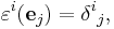
where the right-hand side is the Kronecker delta array. For every covector α in V∗ there exists a unique array of components αi such that

More generally, every tensor T in Tmn(V) has a unique representation in terms of components, meaning that there exists a unique array of scalars Ti1...imj1...in such that

This passage to components forms the bridge between the abstract mathematical notation for tensors, and the way they are commonly written in theoretical physics and engineering texts. More does need to be said, since tensor notation given component-wise only captures part of the idea that a tensor is a "geometric quantity": it covers the aspect of "quantity" but is silent on the geometry. The following explains what happens when a change is made to a different frame of reference, say

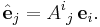
Any two frames are uniquely related, by an invertible transition matrix  , having the property that for all values of
  there holds the frame transformation rule
Let v in V be a vector, and let vi and  denote the corresponding component arrays relative to the two frames. From

and from the frame transformation rule is inferred the vector transformation rule

where Bij is the matrix inverse of Aij, i.e.,

Thus, the transformation rule for a vector's components is contravariant to the transformation rule for the frame of reference. It is for this reason that the superscript indices of a vector are called contravariant.
To establish the transformation rule for covectors, use the transformation rule for the dual basis in the form

Then

while

The transformation rule for covector components is covariant. What this means is the following:  be a given covector, and let
  and
and  be the corresponding component arrays. Then

The above relation is easily established because

and

then use the transformation rule for the frame of reference.
In light of the above discussion, the transformation rule for a general type (m,n) tensor takes the form

In summary, the compatibility of the two standard approaches to tensors means that this component-wise approach, and the abstract mathematics of tensor products introduced in this section, express the same content in two different ways.
Applications
Tensors are important in physics and engineering. In the field of diffusion tensor imaging, for instance, a tensor quantity that expresses the differential permeability of organs to water in varying directions is used to produce scans of the brain; in this technique tensors are in effect made visible. That application is of a tensor of second order. While such uses of tensors are the most frequent, tensors of higher order also matter in many fields.
Continuum mechanics
Important examples are provided by continuum mechanics. The stresses inside a solid body or fluid are described by a tensor. The stress tensor and strain tensor are both second order tensors, and are related in a general linear elastic material by a fourth-order elasticity tensor. In detail, the tensor quantifying stress in a 3-dimensional solid object has components that can be conveniently represented as a 3×3 array. The three faces of a cube-shaped infinitesimal volume segment of the solid are each subject to some given force. The force's vector components are also three in number. Thus, 3×3, or 9 components are required to describe the stress at this cube-shaped infinitesimal segment. Within the bounds of this solid is a whole mass of varying stress quantities, each requiring 9 quantities to describe. Thus, a second order tensor is needed.
If a particular surface element inside the material is singled out, the material on one side of the surface will apply a force on the other side. In general, this force will not be orthogonal to the surface, but it will depend on the orientation of the surface in a linear manner. This is described by a tensor of type (2,0), in linear elasticity, or more precisely by a tensor field of type (2,0), since the stresses may vary from point to point.
Other examples from physics
Common applications include
- Electromagnetic tensor (or Faraday's tensor) in electromagnetism
- Finite deformation tensors for describing deformations and strain tensor for strain in continuum mechanics
- Permittivity and electric susceptibility are tensors in anisotropic media
- Stress-energy tensor in general relativity, used to represent momentum fluxes
- Spherical tensor operators are the eigenfunctions of the quantum angular momentum operator in spherical coordinates
- Diffusion tensors, the basis of Diffusion Tensor Imaging, represent rates of diffusion in biologic environments
Applications of tensors of order > 2
The concept of a tensor of order two is often conflated with that of a matrix. Tensors of higher order do however capture ideas important in science and engineering, as has been shown successively in numerous areas as they develop. This happens, for instance, in the field of computer vision, with the trifocal tensor generalizing the fundamental matrix.
The field of nonlinear optics studies the changes to material polarization density under extreme electric fields. The polarization waves generated are related to the generating electric fields through the nonlinear susceptibility tensor. If the polarization P is not linearly proportional to the electric field E, the medium is termed nonlinear. To a good approximation (for sufficiently weak fields, assuming no permanent dipole moments are present), P is given by a Taylor series in E whose coefficients are the nonlinear susceptibilities:

Here  is the linear susceptibility,
  gives the Pockels effect and second harmonic generation, and
  gives the Kerr effect. This expansion shows the way higher-order tensors arise naturally in the subject matter.
Generalizations
Tensor densities
It is also possible for a tensor field to have a "density". A tensor with density r transforms as an ordinary tensor under coordinate transformations, except that it is also multiplied by the determinant of the Jacobian to the rth power.[14] Invariantly, in the language of multilinear algebra, one can think of tensor densities as multilinear maps taking their values in a density bundle such as the (1-dimensional) space of n-forms (where n is the dimension of the space), as opposed to taking their values in just R. Higher "weights" then just correspond to taking additional tensor products with this space in the range.
In the language of vector bundles, the determinant bundle of the tangent bundle is a line bundle that can be used to 'twist' other bundles r times. While locally the more general transformation law can indeed be used to recognise these tensors, there is a global question that arises, reflecting that in the transformation law one may write either the Jacobian determinant, or its absolute value. Non-integral powers of the (positive) transition functions of the bundle of densities make sense, so that the weight of a density, in that sense, is not restricted to integer values.
Restricting to changes of coordinates with positive Jacobian determinant is possible on orientable manifolds, because there is a consistent global way to eliminate the minus signs; but otherwise the line bundle of densities and the line bundle of n-forms are distinct. For more on the intrinsic meaning, see density on a manifold.)
Spinors
Starting with an orthonormal coordinate system, a tensor transforms in a certain way when a rotation is applied. However, there is additional structure to the group of rotations that is not exhibited by the transformation law for tensors: see orientation entanglement and plate trick. Mathematically, the rotation group is not simply connected. Spinors are mathematical objects that generalize the transformation law for tensors in a way that is sensitive to this fact.
See also
- Glossary of tensor theory
Notation
- Abstract index notation
- Einstein notation
- Voigt notation
- Mandel notation
- Penrose graphical notation
- Raising and lowering indices
Foundational
- Covariance and contravariance of vectors
- Fibre bundle
- One-form
- Tensor field
- Tensor product
- Tensor product of modules
Applications
- Covariant derivative
- Application of tensor theory in engineering
- Curvature
- Diffusion tensor MRI
- Einstein field equations
- Fluid mechanics
- Riemannian geometry
- Tensor derivative
- Tensor decomposition
- Structure Tensor
- Tensor software
Notes
- ↑ This article will be using the term order, since the term rank has a different meaning in the related context of matrices.
- ↑ There is a plethora of different terminology for this around. The terms order, type, rank, valence, and degree are in use for the same concept. This article uses the term "order" or "total order" for the total dimension of the array (or its generalisation in other definitions) m in the preceding example, and the term type for the pair giving the number contravariant and covariant indices. A tensor of type (n,m-n) will also be referred to as a "(n,m-n)" tensor for short.
References
- General
- Bishop, Richard L.; Samuel I. Goldberg (1980) [1968]. Tensor Analysis on Manifolds. Dover. ISBN 978-0-486-64039-6.
- Danielson, Donald A. (2003). Vectors and Tensors in Engineering and Physics (2/e ed.). Westview (Perseus). ISBN 978-0-8133-4080-7.
- Lawden, D. F. (2003). Introduction to Tensor Calculus, Relativity and Cosmology (3/e ed.). Dover. ISBN 978-0-486-42540-5.
- Lebedev, Leonid P.; Michael J. Cloud (2003). Tensor Analysis. World Scientific. ISBN 978-981-238-360-0.
- Lovelock, David; Hanno Rund (1989) [1975]. Tensors, Differential Forms, and Variational Principles. Dover. ISBN 978-0-486-65840-7.
- Munkres, James, Analysis on Manifolds, Westview Press, 1991. Chapter six gives a "from scratch" introduction to covariant tensors.
- Ricci, Gregorio; Levi-Civita, Tullio (March 1900). "Méthodes de calcul différentiel absolu et leurs applications". Mathematische Annalen (Springer) 54 (1–2): 125–201. doi:10.1007/BF01454201. http://www.springerlink.com/content/u21237446l22rgg7/fulltext.pdf
- Kay, David C (1988-04-01). Schaum's Outline of Tensor Calculus. McGraw-Hill. ISBN 978-0070334847.
- Schutz, Bernard, Geometrical methods of mathematical physics, Cambridge University Press, 1980.
- Synge JL, Schild A (1978-07-01). Tensor Calculus. Dover Publications. ISBN 978-0486636122.
- Specific
- ↑ 1.0 1.1 Kline, Morris (1972). Mathematical thought from ancient to modern times, Vol. 3. Oxford University Press. pp. 1122–1127.
- ↑ Karin Reich, Die Entwicklung des Tensorkalküls (1994).
- ↑ William Rowan Hamilton, On some Extensions of Quaternions
- ↑ Namely, the norm operation in a certain type of algebraic system (now known as a Clifford algebra).
- ↑ Woldemar Voigt, Die fundamentalen physikalischen Eigenschaften der Krystalle in elementarer Darstellung (Leipzig, 1898)
- ↑ In volume XVI of the Bulletin des Sciences Mathématiques.
- ↑ Abraham Pais, Subtle is the Lord: The Science and the Life of Albert Einstein
- ↑ Judtih R. Goodstein, The Italian Mathematicians of Relativity (2007)
- ↑ Marion, J.B.; Thornton, S.T. (1995). Classical Dynamics of Particles and Systems (4th ed.). Saunders College Publishing. p. 424. ISBN 9780030989674.
- ↑ Griffiths, D.J. (1999). Introduction to Electrodynamics (3 ed.). Prentice Hall. p. 11--12 and 535--. ISBN 9780138053260.
- ↑ Lee, J.M. (1997). Riemannian Manifolds. Springer. p. 12. ISBN 0387983228.
- ↑ Carroll, S.M. (2004). Spacetime and Geometry. Addison Wesley. p. 21. ISBN 0805387323.
- ↑ Hazewinkel, Michiel, ed. (2001), "Affine tensor", Encyclopaedia of Mathematics, Springer, ISBN 978-1556080104, http://eom.springer.de/a/a011120.htm
- ↑ Hazewinkel, Michiel, ed. (2001), "Tensor density", Encyclopaedia of Mathematics, Springer, ISBN 978-1556080104, http://eom.springer.de/T/t092390.htm
This article incorporates material from tensor on PlanetMath, which is licensed under the Creative Commons Attribution/Share-Alike License.
External links
- Weisstein, Eric W., "Tensor" from MathWorld.
- Introduction to Vectors and Tensors, Vol 1: Linear and Multilinear Algebra by Ray M. Bowen and C. C. Wang.
- Introduction to Vectors and Tensors, Vol 2: Vector and Tensor Analysis by Ray M. Bowen and C. C. Wang.
- An Introduction to Tensors for Students of Physics and Engineering, released by NASA
- A discussion of the various approaches to teaching tensors, and recommendations of textbooks
- A Quick Introduction to Tensor Analysis by R. A. Sharipov.
- Introduction to Tensors by Joakim Strandberg.